Using Instrument Nonlinear Correction (INC)

The instrument will provide one or two types of nonlinear corrections correction using Digital Predistortion (DPD) technique based on the model number. All instruments provide DUT Nonlinear Correction to predistort the signal applied to the Device Under Test, which primarily targets Power Amplifier testing. The algorithm for DUT Nonlinear Correction is compatible with the Keysight N7614C Signal Studio for Power Amplifier Test.

For M9383B, M9384B, and M9484C, with N7653APPC subscription date of 2020.1215 or later, provides Instrument Nonlinear Correction, which compensates the instrument’s nonlinearity

How it Works

Applying digital predistortion (DPD) to your waveform is a two-step process. You must first enable nonlinear correction and then enable vector modulation, which initiates both the DPD calculation and waveform upload operations. The IQ data is therefore modified during the upload process, creating the predistorted waveform that will reside in the signal generator's volatile (arb) memory.

Digital Predistortion (DPD) is applied to the waveform before uploading it to the arb memory. For example, when DUT Nonlinear Correction is enabled, the signal generator internally creates the predistorted waveform as a part of the waveform uploading operation. Therefore, the predistorted waveform is not saved in the non-volatile memory.

Note that the predistortion calculation doesn’t run unless Signal upload occurs. For example, the waveform is not uploaded when Enable Vector Modulation Signal is off. Which means no DPD calculation runs at this moment. When Enable Vector Modulation Signal is checked (turned on), the waveform upload is triggered and DPD is applied as a part of the upload sequence.It should also be noted that DPD cannot be applied to a waveform already in the arb memory. This is because IQ data in the arb memory cannot be modified on the signal generator.

Calibration and Correction Concepts

An Instrument Nonlinear Correction (INC) calibration can improve the characteristics of the signal generated by digitally predistorting the waveform to reduce distortion components. In order to perform a successful INC calibration and correction, the generated signal must have significant distortion components which are measurable (can be differentiated from the noise floor). If this is not the case, then the quality of the signal cannot be improved. The resulting corrected waveform should always be examined to verify the desired signal improvements were achieved.

The calibration process utilizes an external receiver, typically a spectrum analyzer (connected to the source via cabling and potentially other components), for iteratively measuring and distorting an output signal in order to determine a correction model. This model is then applied to the original waveform to achieve a predistorted corrected waveform which, when played, will exhibit improved signal characteristics.

The INC calibration process consists of two parts: the measurement phase, and the correction phase. At the beginning of the measurement phase, the initial waveform used for the distortion process is determined. The measurement phase then performs an iterative process of measuring this waveform then distorting it. This iteration continues until either a maximum number of iterations has been reached, or the measured results are within specified tolerances. The result of the measurement phase is a waveform that has been distorted to optimize the desired signal characteristics. The correction phase then calculates a memory-model, which is then applied to the original waveform to generate the corrected waveform.

The INC calibration process generates an INC file with a file name based on the selected waveform file name with an ".inc" extension. The generated INC file name is the same as the selected waveform file name plus an additional channel indicator, "C<channel-number>", in order to help differentiate INC files by the channel that was used for the calibration. For example, if the selected waveform file name were Qam16Bw500MHz.wfm, and the INC calibration were performed using Channel 1, then the resulting INC file name would be Qam16Bw500MHzC1.wfm.

The INC file contains all the information related to the calibration process, including the original waveform, the instrument state, the memory-model, and the corrected waveform. The instrument recognizes INC files via the ".inc" extension. Once an INC file is selected, the instrument can be easily configured to playback the original waveform, playback the corrected waveform, re-establish the instrument state, and refresh the INC file. Any supported waveform type can be corrected via the INC calibration. The result is always an .inc file.

The calibration process corrects for linear and/or nonlinear effects in the system; such effects are hardware specific. Consequently, an INC file should only be utilized for the same instrument, and channel of the instrument, that the calibration process utilized when generating the INC file. Furthermore, the linear and nonlinear effects are dependent upon the state of the instrument at the time of the calibration. In order to preserve optimal signal characteristics when playing a corrected waveform, the instrument state needs to be restored to what existed at the time of the calibration. Note that the instrument settings can deviate from the calibrated state, but performance will degrade. To help mitigate this, multiple INC files can be generated on the same original waveform file at different carrier frequencies and power levels. Additionally, periodically re-calibrating existing INC files is recommended to take into account temperature and instrument drift.

To recalibrate an INC file, select the INC file, restore the state (use Recall Calibrated State), disable the INC correction (switch the source to play the original waveform), then perform the calibration (the calibration parameters are fully restored). Note that a receiver must be properly connected to the source. This will update the INC file with the latest correction data and corrected waveform.

In order to reduce the calibration time, the original waveform can be compacted; this generates a compacted waveform with the same spectral qualities as the original, but with significantly fewer samples. Using compaction significantly reduces the calibration time; however, for some signals, the best compaction level may need to be experimentally determined. By default, the compaction level is calculated and this results in the measurement phase of the calibration process utilizing and distorting the compacted waveform. This also means that the generated memory-model is based on the initial compacted waveform and the final distorted compact waveform. For many cases of waveforms, the resulting corrected waveform (from applying the memory-model to the original waveform) will yield improved signal characteristics. However, in some cases, it may be desirable to avoid compaction. Thus the measurement phase and memory-model generation are done using the full waveform. The downside is a longer calibration time (in some cases the calibration process may take hours).

The memory-model stored in an INC file can be applied to other waveform files, and this will similarly generate an INC file. However, this process, while considerably faster and not requiring a receiver, should only be done when the waveform being corrected is similar to the original waveform used to generate the memory-model, and where the original calibration settings used are also appropriate. The new INC file contains the instrument state and memory-model from the original INC file, the new original waveform, and the new corrected waveform generated by applying the memory-model to the new original waveform.

Calibration Overview

The result of a calibration process is an .inc file, which the source can utilize similarly to other waveform file types. There are several calibration choices which affect the measurement phase of the calibration process, and therefore the signal characteristics of the corrected waveform. Effective combinations of the following choices typically include at least one linear or nonlinear calibration coupled with Power calibration. Note that utilizing all of the following calibrations is supported and generally recommended:

Power: If enabled at the beginning of the measurement phase, the power of the signal at the input to the receiver will be adjusted to achieve a specified power level. This choice can be used to compensate for gain or loss of external components connected to the output of the source. This calibration does not affect the waveform itself; it only affects the power setting of the source.
Equalization: If enabled, the waveform is measured (once) and distorted such that the magnitude and phase of the output signal best matches the original waveform. This calibration corrects for only linear effects in the system and is applied to the initial waveform prior to utilizing a memory-model.
Distortion (EVM): If enabled, this calibration iteratively measures and distorts the waveform (either full or compacted) until either the maximum number of iterations has been reached or the measured EVM of the distorted waveform is equal to or better than the specified EVM (which is the tolerance for this calibration). The initial and final waveforms are then used to generate the memory-model which is applied to the original waveform to generate the corrected waveform. Note that the Equalization calibration is always performed as part of the Distortion (EVM) calibration.
Adjacent Channel Power (ACP): If enabled, the power in the specified regions above and below the modulated signal is reduced in an iterative process until either the maximum number of iterations is reached, or the measured ACPR in the ACP regions is below the specified level (which is the tolerance for this calibration). This calibration also affects the initial and final waveforms and consequently affects the memory-model. Additionally, this calibration increases the number of samples in the waveform, changes the sample rate, and the playback duration of the corrected waveform from what existed for the original waveform.

An INC calibration requires these steps:

Connect the RF input of the receiver to an RF output on the source via cables and potentially other components.
Connect the 10-MHz reference output from the source to the 10 MHz reference input of the receiver.
Configure the source to generate the desired signal at the target output power and carrier frequency.
Configure the INC calibrations to be performed (including all calibration-related parameters and the IO connection to the receiver).

As a minimum configuration, at least one of Distortion (EVM), Equalization, or ACP must be selected in order to perform an INC calibration (otherwise, a corrected waveform and the INC file cannot be generated).
Initiate the calibration. The source will control the receiver to perform the necessary measurements, then perform the necessary calculations to generate an .inc file. After the .inc file is generated, the calibration process configures the source to playback the corrected waveform from the .inc file.
The receiver can be used to determine the results of the calibration process (performed manually by the user). In some cases, the advanced calibration parameters may need to be adjusted to achieve optimal results.

Depending on the calibration parameters and the characteristics of the uncorrected waveform, a calibration may take as little as a few minutes, to a significant portion of an hour (or greater).

Basic Calibration Configuration

When performing an INC calibration from the GUI, a dialog is shown that provides the option to abort the process. When an INC calibration is initiated from SCPI, the process is synchronous, and no abort mechanism is supported.

Each of the calibrations mentioned in the previous section need to be configured, as outlined below:

Power Calibration

The Power calibration adjusts the source output power to achieve a desired power level at the input to the receiver, which compensates for loss or gain due to components that are used to connect the source to the receiver. This calibration is accessed from the Calibrations tab of the Instrument Nonlinear Calibration screen and is enabled by marking the associated checkbox. (SCPI operation is also provided.) The following parameters should be configured for basic operation of this calibration:

Adjust the Nominal Cable Gain and Failsafe Max Power in the Advanced tab.

Nominal Cable Gain reflects the expected loss or gain due to the components that connect the source to the receiver. For example, if the cable loss at the carrier frequency is 1.8 dB, then enter -1.8. This setting is used with the RF output power setting to calculate a reasonable initial source power level at the beginning of the power calibration.

Failsafe Max Power limits the source power during the power calibration. For example, if this value is set to 10 dBm, then the maximum power the source will be set to is 10 dBm.
Enter the desired signal power level that the receiver should measure for the RF output power. For example, if the desired output power is 0 dBm then enter 0 for the RF Output Power of the source channel being calibrated.
In the Calibrations Tab do the following:
1. Mark the Power checkbox, or use the corresponding SCPI command, to enable the power calibration.
2. Specify the Span, if necessary. Note that the span setting for Equalization, Distortion (EVM), and Power calibrations are coupled, so this value only needs to be entered for one of these calibrations. Typically, the span setting should be the occupied bandwidth of the waveform.
3. Enter the maximum number of iterations and the tolerance for the power calibration. The power calibration will iterate, each iteration adjusts the source output power closer to the desired power level (as measured by the receiver). The power calibration will stop once the difference between the measured power and desired output power is less than the tolerance, or the maximum number of iterations has been reached.
Once all of the settings are configured, the calibration process can be started via the Start Calibration button or corresponding SCPI command.

An INC calibration cannot be performed if only a power calibration is enabled. An INC calibration process always generates an INC file that contains a corrected waveform, and the power calibration itself does not result in a corrected waveform. The result of the power calibration is only a value change to the power offset setting of the channel being calibrated.

Equalization Calibration

The Equalization calibration performs an equalization correction on the waveform used in the measurement phase of the calibration. The generated signal is distorted such that the magnitude and phase (as measured by the receiver) match the original waveform via a spline-fitting algorithm. This is only a linear correction of the original waveform, and does not utilize an iterative process based on optimizing the signal EVM. However, Equalization is not as time consuming as the full Distortion (EVM) calibration. Configure the equalization calibration as follows:

Mark the Equalization checkbox, or use the corresponding SCPI command, to enable the equalization calibration.
Specify the Span, if necessary. Note that the span setting for Equalization, Distortion (EVM), and Power calibrations are coupled, so this value only needs to be entered for one of these calibrations. Typically, the span setting should be the occupied bandwidth of the waveform.
Once all of the settings are configured, the calibration process can be started via the Start Calibration button or corresponding SCPI command.

The Equalization calibration will generate an INC file with a corrected waveform file as well as a memory model.

Distortion (EVM) Calibration

The Distortion (EVM) calibration is a comprehensive calibration process that improves the EVM of a signal. This calibration utilizes the Equalization calibration to perform a linear correction, and a nonlinear distortion process that iteratively improves the EVM of the signal. The nonlinear portion distorts the signal iteratively to improve the EVM. Generally, when using waveform compaction, using both equalization and distortion (EVM) calibration yield the best results. Configure the distortion (EVM) calibration as follows:

Mark the Distortion (EVM) checkbox, or use the corresponding SCPI command, to enable the distortion (EVM) calibration. This will also visually enable the Equalization calibration in the GUI to reflect that the Distortion (EVM) calibration is a superset of Equalization.
Specify the Span, if necessary. Note that the span setting for Equalization, Distortion (EVM), and Power calibrations are coupled, so this value only needs to be entered for one of these calibrations. Typically, the span setting should be the occupied bandwidth of the waveform.
Specify the tolerance and max iterations. The tolerance for the distortion (EVM) calibration is the target EVM for the distorted waveform. Note that if compaction is used, then the distorted waveform is based on a compacted waveform, otherwise it is based on the original waveform. Note that the measured EVM of a distorted waveform may vary from the measured EVM of the original waveform or the final corrected waveform. Max iterations specifies the maximum number of iterations that will be allowed if the tolerance is not achieved.
Once all of the settings are configured, the calibration process can be started via the Start Calibration button or corresponding SCPI command.

The EVM of multi-channel waveforms can be improved via Distortion (EVM) calibration. In these cases, the Span should be set to the bandwidth of the combined channels (including the channel separation). For example, if a two-channel signal is being corrected where each channel is 50 MHz with a 50 MHz separation between channels, then the Span should be set to 150 MHz. In these cases, the Distortion (EVM) calibration can reduce the noise in the channel separation region provided sufficient averaging is used. If the resulting noise level is too high, try increase the averaging.

Adjacent Channel Power (ACP) Calibration

The ACP calibration is an iterative correction which reduces the power in regions above and below the modulated signal bandwidth. Configure the ACP calibration as follows:

Mark the ACP checkbox, or use the corresponding SCPI command, to enable the ACP calibration.
Specify the Span of the ACP regions. The power in two regions, one above and the other below the modulated signal bandwidth will be minimized by the calibration. The span is the bandwidth of these regions (each region has the same span, or bandwidth).
Specify the Offset frequency of each of these regions. The actual center frequency of each region is the carrier frequency +/- the offset frequency. For example, if the carrier frequency is 30 GHz, and the occupied bandwidth of the signal is 800 MHz, and the desired ACP region is 500 MHz wide, just above and below the signal, then:
1. Source Output Frequency should be set to 30 GHz
2. Distortion (EVM) or Power or Equalization Span should be set to 800 MHz
3. ACP Span should be set to 500 MHz
4. ACP Offset should be set to (800 / 2 + 500 / 2) MHz or 650 MHz
Specify the tolerance and max iterations. The tolerance for the ACP calibration is the target NPR or ACP in units of dBc that is measured in the ACP regions Note that if compaction is used, then the distorted waveform is based on a compacted waveform, otherwise it is based on the original waveform. The max iterations specify the maximum number of iterations that will be allowed if the measured NPR or ACP is not below the specified tolerance.
Once all of the settings are configured, the calibration process can be started via the Start Calibration button or corresponding SCPI command.

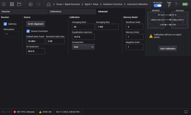
Advanced Calibration Configuration

The Advanced tab is organized into four groups of related settings:

Receiver settings
Source settings
Calibration settings
Memory Model settings

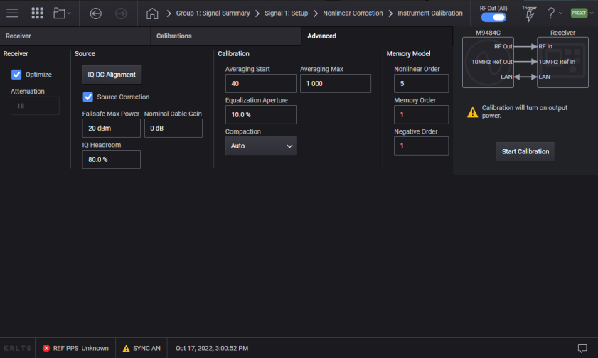
Receiver

When the Receiver Optimization checkbox is marked, the calibration process will automatically determine the optimal receiver attenuation, IF gain state, and IF gain to use to achieve the best measurement fidelity. In some situations, you may want to specify these settings manually, in which case the checkbox should be unmarked and you can specify the values.

Improper setup can result in ADC overrange errors in the receiver during the calibration measurement phase, which will cause the calibration process to terminate prematurely with an error.

When receiver optimization is enabled, receiver ADC overrange errors may be observed, this is normal as the optimization algorithm determines the best levels for these settings. Once the optimization has completed, no further ADC overrange errors should occur.

Source

When the Source Correction checkbox is marked, the calibration process will utilize certain optimizations and/or corrections of the source. Currently, this is limited to the source flatness correction, and the optimize dynamic range with OBW. Thus, when Source Correction is enabled, both source flatness correction and optimized behavior for dynamic range will be enabled during the calibration. When playing the corrected waveform, these source settings should be set up to match what was done during the calibration, otherwise the fidelity of the corrected signal will be compromised. This is one example (of many) why the calibrated state should be restored when playing the corrected waveform.

The Failsafe Max Power entry specifies the maximum output power that will be set by the power calibration. This is to prevent overdriving a DUT with excessive power during a power calibration or subsequent calibration process.

The Nominal Cable Gain entry allows the user to provide an estimated gain or loss to compensate for the components (cables, amplifiers, attenuators, etc.) which are used to connect the source to the receiver.

At the beginning of the power calibration, the source power starts at:

Initial source power = RF Output Power – Nominal Cable Gain.

As the power calibration iterates, the RF output power is adjusted until the power measured by the receiver matches the power setting of the source.

For example, if the source output power setting is 0 dBm, and a cable with 3 dB of loss is used to connect the source to the receiver, and Nominal Cable Gain were set to -3 dB, the initial iteration of the power calibration would start at 3 dBm output power from the source, and the receiver will measure approximately 0 dBm (desired power level achieved in one iteration). At the conclusion of the power calibration, the receiver will measure 0 dBm of power, the RF output power will be 3 dB plus or minus the actual cable loss within the tolerance specified.

The calibration process will reduce the magnitude of the IQ data in the playing waveform in order to allow for expansion of peaks as the waveform is distorted. The amount of this scaling is specified by the IQ Headroom setting and is a percent of the full DAC range.

At the beginning of the calibration process, the initial distorted waveform is scaled by the IQ Headroom. If this value is too high, DAC overrange errors will result during the calibration process (which will terminate prematurely). In this case, there are a couple of actions which can resolve the problem:

Decrease the IQ Headroom (first choice).
Decrease the waveform Scale.

Calibration

Averaging Start and Averaging Max: during the calibration process the averaging dynamically changes and these settings allow tuning the initial and maximum averaging used during the calibration process.

The Equalization Aperture entry allows specifying the percentage of the distortion (EVM) span to be used in the equalization spline.

The calibration process is typically performed using a compacted waveform which is generated using a fraction of the IQ data from the uncorrected waveform (number of samples in compacted waveform = number of samples in original waveform / compaction). The higher the compaction, the fewer IQ samples in the distorted waveform and this reduces the calibration time. However, this can adversely affect the quality of the memory model and resulting corrected waveform because as the compaction increases, so does the difference in the spectral qualities between the compacted and original waveforms. The Compaction-Auto checkbox, if enabled, results in the calibration process automatically determining the compaction. Unmarking Auto allows you to enter a value for compaction. Specifying a compaction of 1 results in the calibration process utilizing the full original waveform, which may result in an excessive calibration duration.

Memory Model

These settings enable you to configure the properties of the memory model.